5  Pseudorandom number generation

Uniformly distributed random numbers

Uniformly distributed random numbers are generated with runif(n, min, max). Default parameters are n=1, min=0, max=1.

runif(20,-1,1) # 20 random numbers, uniformly distributed between -1 and 1.
 [1]  0.0434271717 -0.2545901961 -0.8550298712  0.1515010367 -0.4330742215
 [6]  0.8933711154 -0.6796927955  0.0004589334  0.1694160644  0.3009928511
[11]  0.2048388137  0.0054464517 -0.3716698317 -0.8119168803  0.0464187078
[16] -0.7662025592  0.4662518837  0.5770013169  0.2459967798 -0.9186255848
runif(20,-1,1) # 20 random numbers, uniformly distributed between -1 and 1.
 [1] -0.43654619  0.57851000 -0.20333654 -0.14091812 -0.03801497 -0.10647906
 [7] -0.64735658 -0.88589618  0.79982700  0.38114682 -0.28573955  0.11965487
[13] -0.49397596  0.35485469 -0.03999775  0.25907603 -0.77256892  0.27046182
[19]  0.76141921 -0.96163945

Normally distributed random numbers

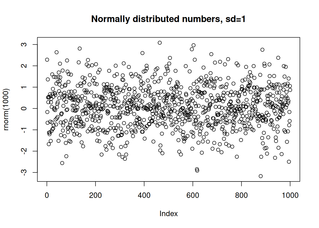
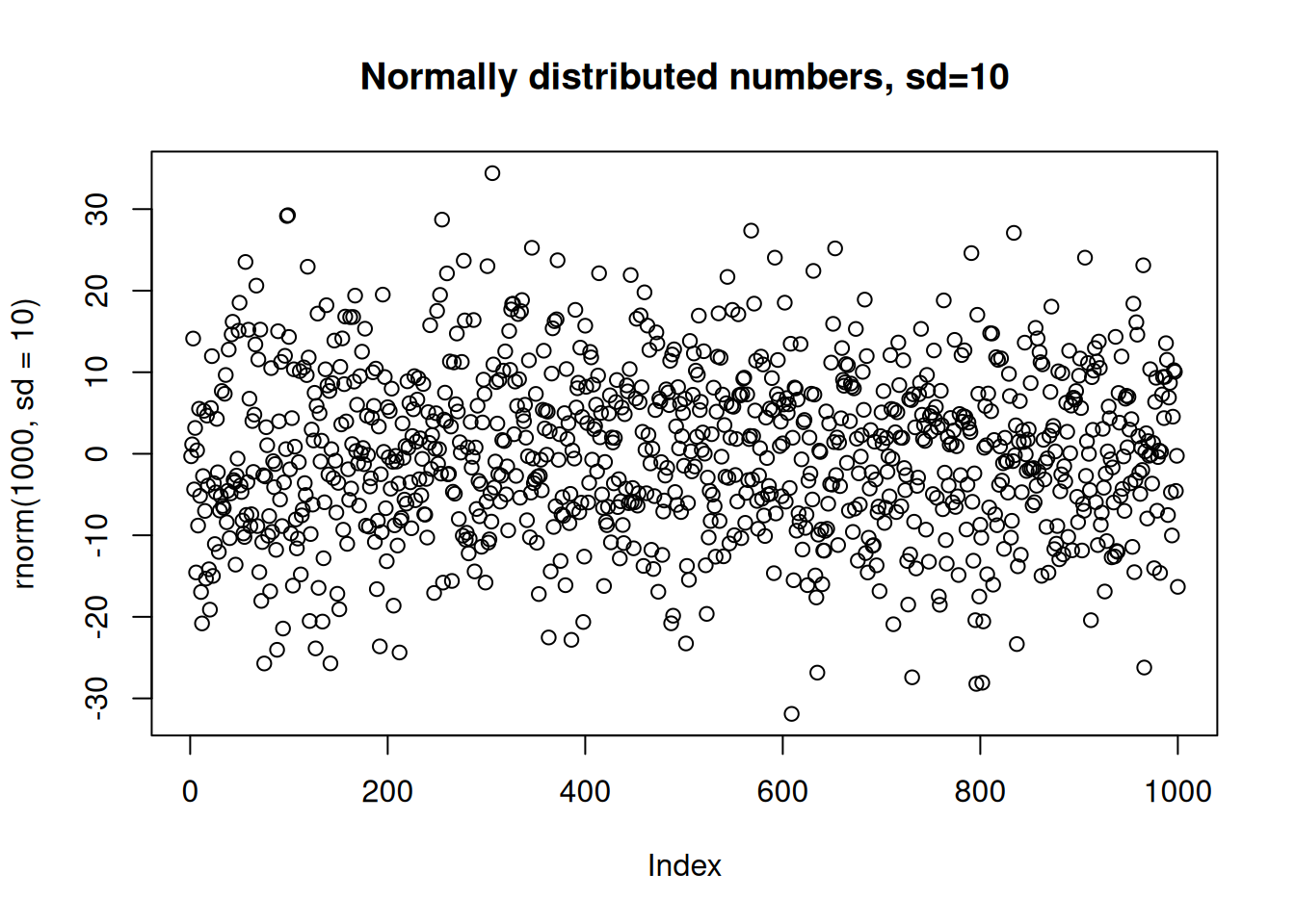
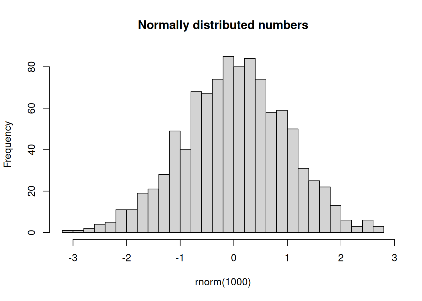
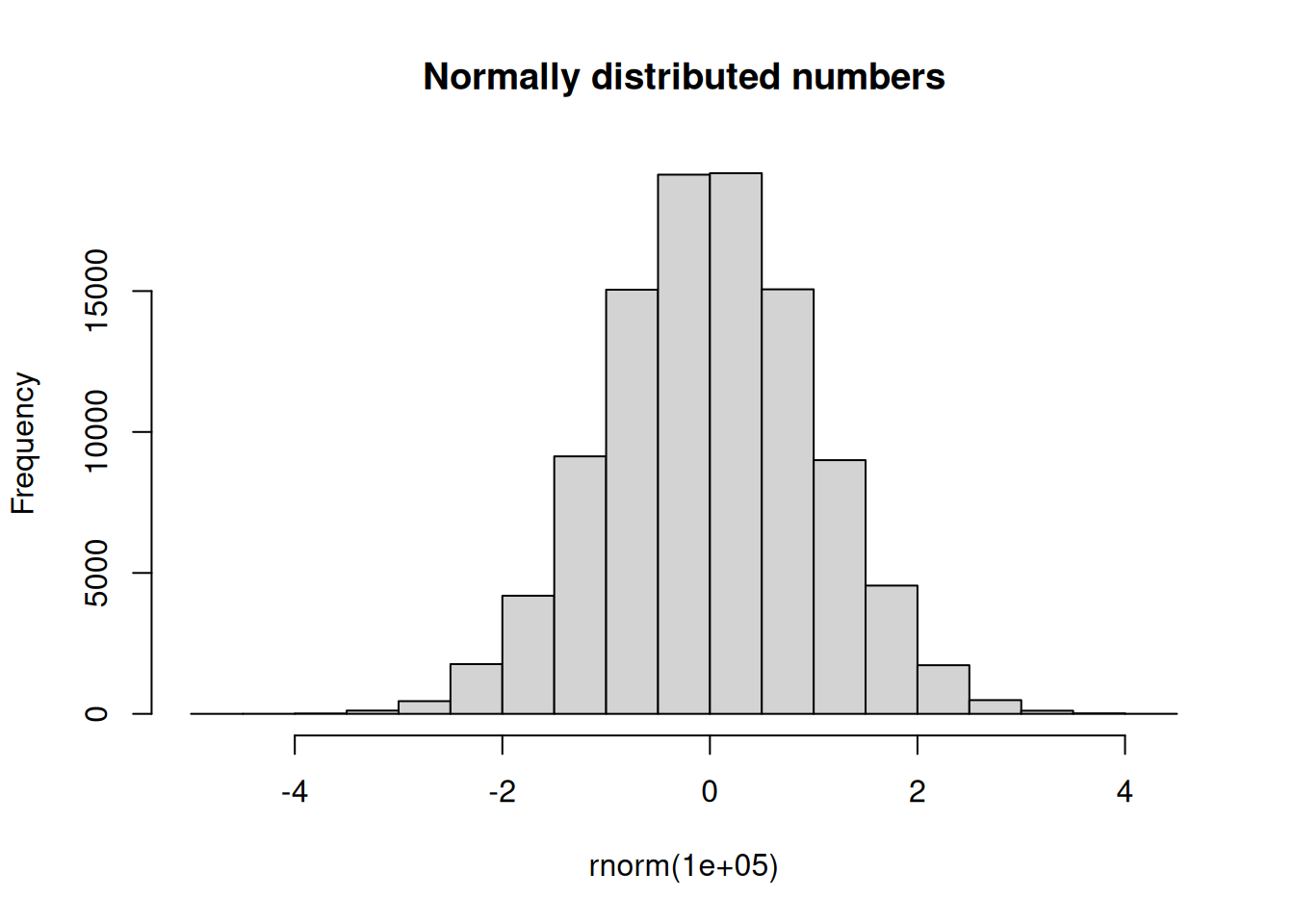
Another common distribution is the Normal or Gaussian distribution (a.k.a. the bell curve). Normally distributed random numbers are generated with the rnorm(n,mean,sd) function. Default parameter values are n=1, mean=0, sd=1.

rnorm(20)
 [1] -1.7464598 -2.5608446 -1.0940751 -0.5922735 -0.2945351 -0.6309478
 [7]  0.8917938  0.5374663  1.0173756 -1.5275702  0.2170979 -0.1413056
[13]  1.7290465 -0.6582857 -0.6587658  1.8619994  0.6325903 -0.6783980
[19]  0.3721694  2.3345917

Comparison of distributions

options(repr.plot.width=8, repr.plot.height=3)
plot(runif(1000,-1,1)); title("Uniformly distributed numbers")

plot(rnorm(1000)); title("Normally distributed numbers, sd=1")

plot(rnorm(1000,sd=10)); title("Normally distributed numbers, sd=10")

Plot the histograms of the random samples.

hist(runif(1000,-1,1), breaks=25, main="Uniformly distributed numbers")

hist(rnorm(1000), breaks=25,main="Normally distributed numbers")

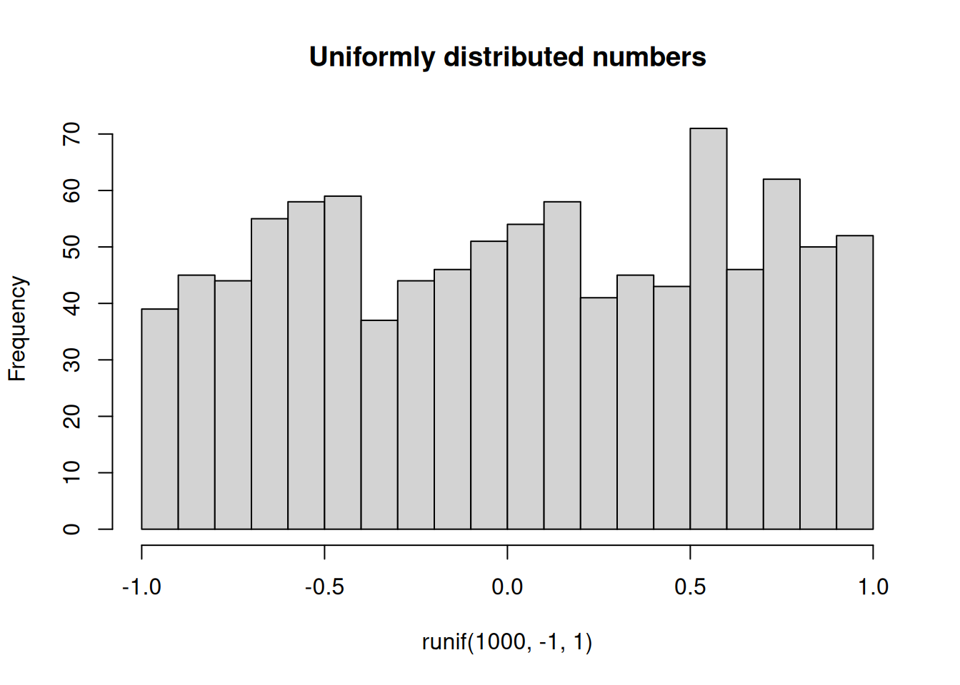
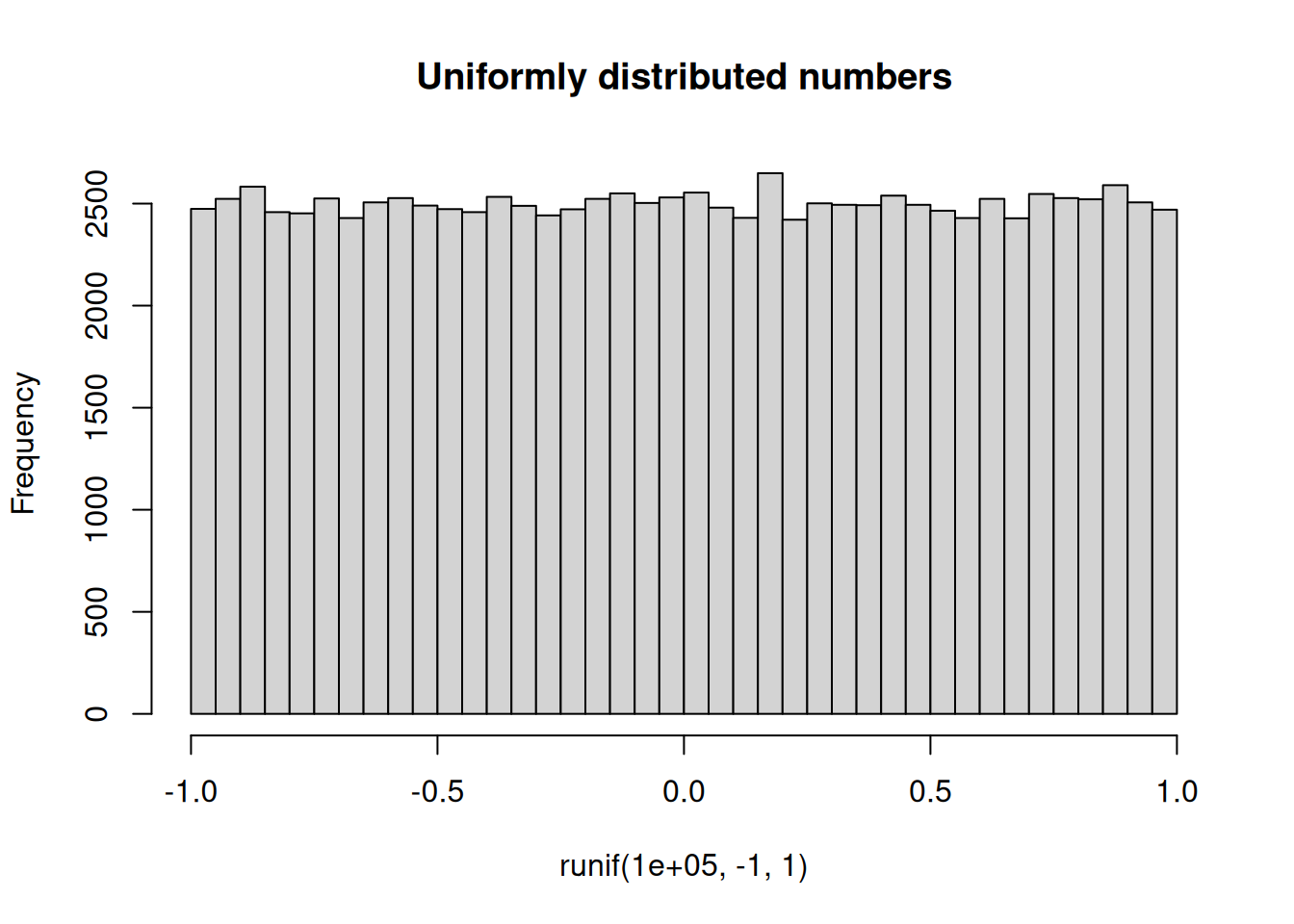
Note that the distributions are not perfectly smooth. The reason is that our random sample is finite. As we draw more and more samples, the histogram will approach the theoretical distribution.

hist(runif(100000,-1,1), breaks=30, main="Uniformly distributed numbers")

hist(rnorm(100000), breaks=30, main="Normally distributed numbers")

Generating synthetic data

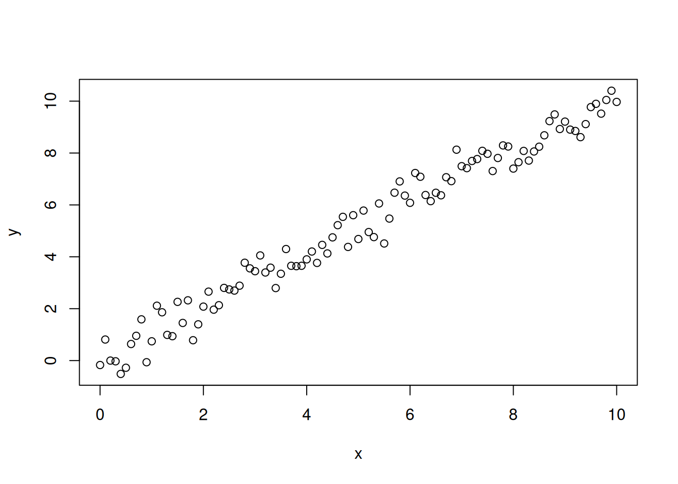
By adding random “noise” to deterministic vectors, we can simulate a real-life data set where the underlying “law” is \(y=x\).

x <- seq(0,10, length.out = 101)
y <- x + rnorm(length(x), sd=0.5)
plot(x,y)

Getting the same random sequence every time

In some cases we want to get the same random sequence in every simulation, so that we can identify and correct errors. For that, we can set the seed of the random number generator to a fixed number.

set.seed(1234)
runif(10,-1,1)
 [1] -0.77259318  0.24459881  0.21854947  0.24675888  0.72183077  0.28062121
 [7] -0.98100849 -0.53489899  0.33216752  0.02850228
set.seed(1234)
runif(10,-1,1)
 [1] -0.77259318  0.24459881  0.21854947  0.24675888  0.72183077  0.28062121
 [7] -0.98100849 -0.53489899  0.33216752  0.02850228

Choosing a vector element randomly

The sample function allows us to selected elements randomly from a given vector.

By default, it chooses elements without replacement. So, an element is chosen at most once.

x <- 11:20
sample(x)
 [1] 14 12 17 16 19 20 18 15 13 11

To choose elements with replacement, we set the replace parameter to TRUE.

sample(x, 10, replace = TRUE)
 [1] 14 14 15 18 14 18 13 14 20 15

Coin toss experiment


tosses <- sample(c("H","T"),size=10,replace = TRUE)
tosses
 [1] "T" "T" "H" "T" "H" "T" "T" "T" "H" "H"

We throw a coin 10 times. How many heads do we get on average?

The number of heads in one experiment (10 throws):

tosses=="H"
 [1] FALSE FALSE  TRUE FALSE  TRUE FALSE FALSE FALSE  TRUE  TRUE
sum(tosses=="H")
[1] 4

This number changes every time due to the randomness:

tosses <- sample(c("H","T"),10,replace = TRUE)
sum(tosses=="H")
[1] 4

In order to get the expected number of heads, we need to repeat the experiment many times and average over the outcomes. (See “loops” later.)

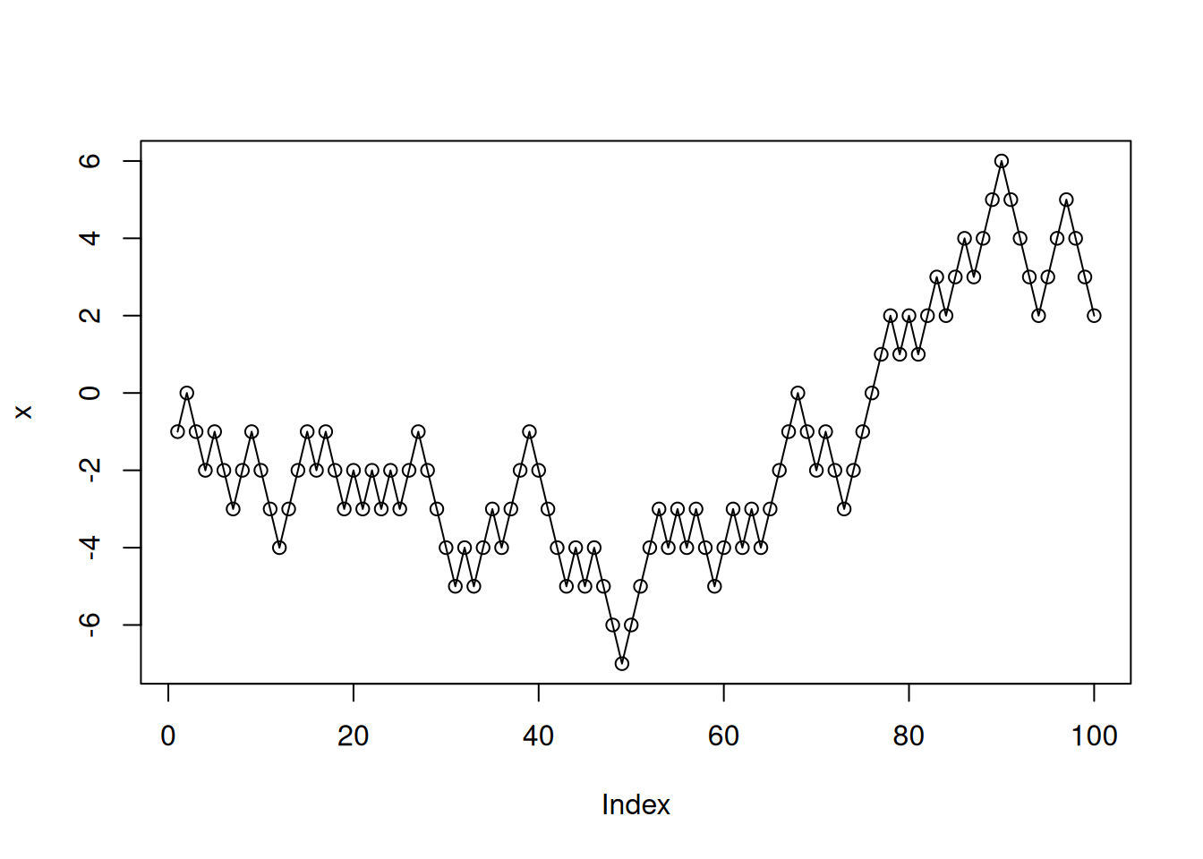
Suppose you gamble with a coin: You gain 1 TL if it comes heads, and lose 1 TL otherwise. You repeat the coin toss 5 times. What is your balance at every step of the game?

Our gain is +1 if heads, and -1 if tails. To simplify the accounting, let us sample from (-1,1) and get the cumulative sum.

outcomes <- sample(c(-1,1), 5, replace=TRUE)
outcomes
[1] -1  1 -1  1  1
cumsum(outcomes)
[1] -1  0 -1  0  1

Repeat the coin toss 100 times. The balance looks as follows.

options(repr.plot.width=10, repr.plot.height=4)
x <- cumsum(sample(c(-1,1), 100, replace=TRUE))
plot(x, type="o")

This is called a random walk.

Throwing dice


d1 <- sample(1:6, 10, replace=TRUE)
d2 <- sample(1:6, 10, replace=TRUE)
d1
 [1] 1 2 6 6 3 6 6 3 5 6
d2
 [1] 6 4 3 3 1 3 4 3 3 2

Simulating the outcome of a pair of dice:

d1 + d2
 [1]  7  6  9  9  4  9 10  6  8  8

Now throw two dice 1000 times and plot a histogram of the total outcomes.

d1 <- sample(1:6, 100000, replace=TRUE)
d2 <- sample(1:6, 100000, replace=TRUE)
hist(d1+d2, breaks = 1:12)

Estimating pi

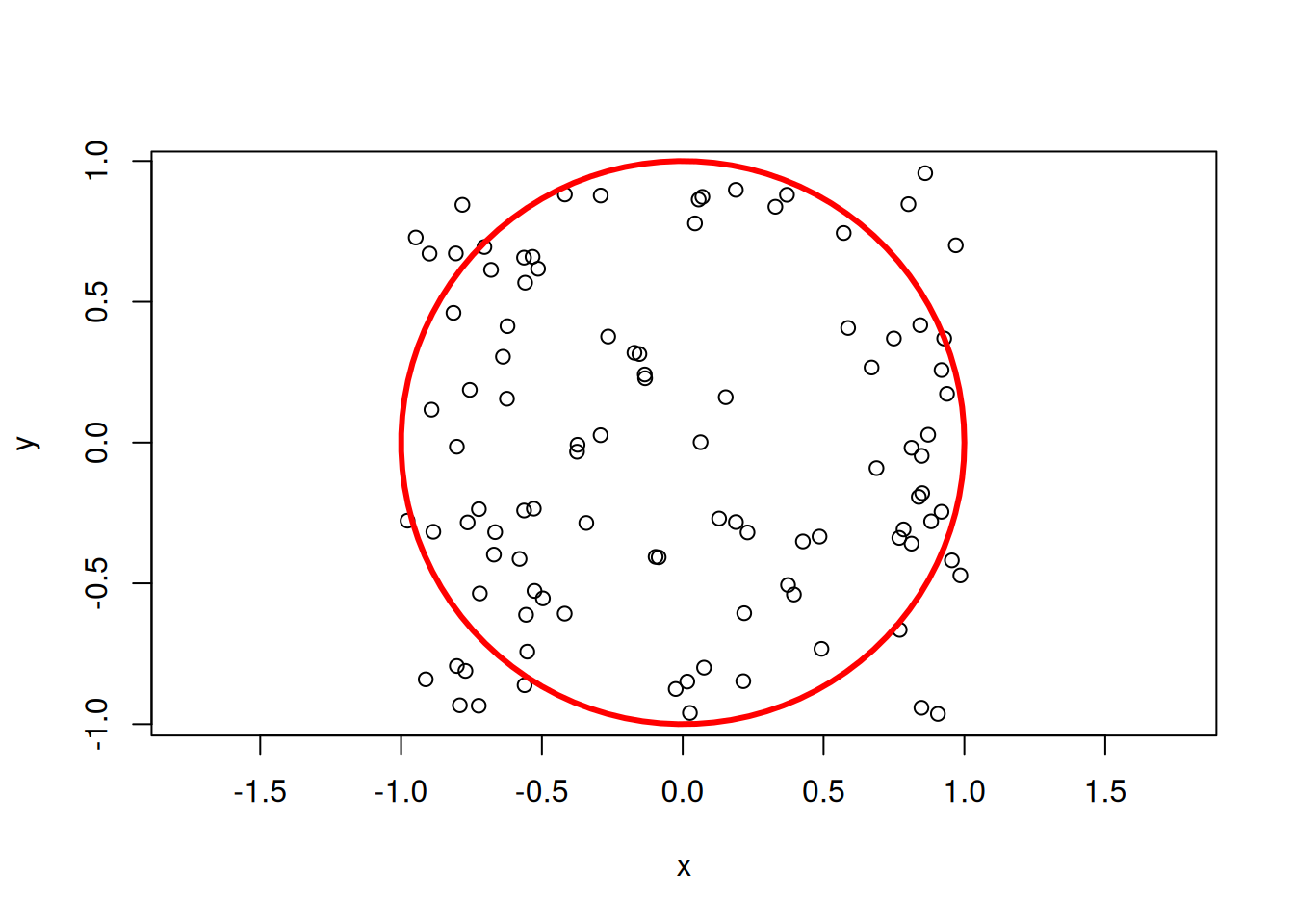
Suppose we generate random number pairs \((x,y)\) within the square \(-1\leq x\leq 1\) and \(-1\leq y\leq 1\). Some of them fall inside the inscribed circle \(x^2 + y^2 \leq 1\).

options(repr.plot.width=4, repr.plot.height=4)
x <- runif(100,-1,1)
y <- runif(100,-1,1)
# plot the random points:
plot(x, y, asp=1)
# plot the unit circle:
t <- seq(0,2*pi, length.out=100)
xx <- cos(t)
yy <- sin(t)
lines(xx,yy,lwd = 3,col="red")

The area of the circle is \(\pi\) and the area of the square is 4, so the ratio of points inside the circle to the points inside the square gives an estimate of \(\pi/4\). So, we can approximate \(\pi\) as:

4*sum(x^2 + y^2 <= 1)/length(x)
[1] 3.24

With a new set of random hits, the estimate will differ:

x <- runif(100,-1,1)
y <- runif(100,-1,1)
4*sum(x^2 + y^2 < 1)/length(x)
[1] 3.16

Exercises

  1. Write an R expression that simulates the outcome of the 6/49 Lottery (Sayısal Loto), where one draws 6 numbers from 1, 2, …, 49. Note that the same number cannot appear twice in one drawing.

  2. Generate 1000 random numbers, drawn from the normal distribution with standard deviation 2, and another 1000 with standard deviation 0.5. Plot the histogram for each set of numbers. What can you say about the effect of the standard deviation?

  3. Throw 10 coins and count the number of heads. Repeat this experiment ten times, and find the mean of the number of heads.

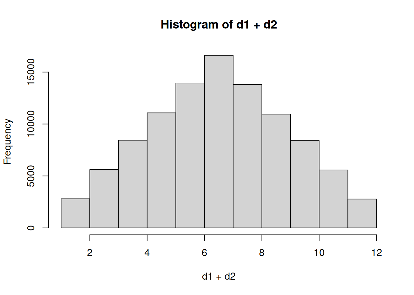
  4. Throw 3 dice 10000 times. Plot the histogram of the outcomes (outcomes should be between 3 and 18).